Introduction

After the most recent H5N1 avian influenza epidemics and during the 2009 H1N1 influenza pandemic, the international scientific community in the public health area has made efforts within the framework of the imperative need to develop standardized research and collect data that will serve as support to face eventual pandemics (Sundus, et al., 2018; Shakeri, et al., 2018; Alzahrani, et al., 2019; Ren-Zhang, et al., 2020). On December 31, 2019, 27 cases of pneumonia of unknown etiology were identified in Wuhan City, Hubei Province in China. Wuhan is the most populous city in central China with a population of over 11 million. These patients presented most notably with clinical symptoms of dry cough, dyspnea, fever, and bilateral pulmonary infiltrates on imaging. All of the cases were related to the Wuhan Huanan Seafood Wholesale Market, which marketed fish and a variety of live animal species, such as poultry, bats, marmots, and snakes (Lu et al. 2020). The causative agent was identified from throat swab samples conducted by the Chinese Center for Disease Control and Prevention (CCDC) on January 7, 2020, and was subsequently named Severe Acute Respiratory Syndrome Coronavirus 2 (SARS- CoV-2). The disease was named COVID-19 by the World Health Organization, known by its Spanish acronym WHO (World Health Organization, 2020).

To apply epidemiological models it is essential to understand the phenomena of complexity and chaos since chaos theory has been considered as a possible underlying explanatory model. The parameters associated with chaos are dimension measurements and information generation rates (entropy), understanding entropy as a measure of disorder. Since these analyses require large series of data that frequently make their calculation very difficult if not impossible in practical terms, theories and methods were devised to make the statistical study of regularity feasible, relating the information generation index with entropy, applied to small series of clinical data originated from complex “noisy” systems to demonstrate the existence or non-existence of chaos and non-linearity (Cuestas, 2013). Beyond the criteria that involve the evaluation of models, from the adjustment coefficient (R2), the entropy (Information criteria), the number of parameters (Mallows' Cp), the residual standard error (ERR), which although they are criteria that allow calibrating the predictive capacity of the model, they are not a sufficient condition for these models to be used as instruments for decision-making. It is the circumstances surrounding the environment of the phenomenon that determine the quality of the information, that is, of the sample, and consequently the levels of entropy of the models.

In the case of COVID-19 in Peru, where on March 6, 2020, the first case of contagion was registered, marking the beginning of a public health problem that has led the Peruvian Government to take measures ranging from social distancing, mandatory social isolation, until mandatory social immobilization, and that to date (April 15, 2020) despite these mediations, the figure stands at more than 11,000 confirmed cases of contagion by COVID-19 in much of the national territory. In this sense, in Peru, the limitations in the acquisition of tests as a consequence of a global phenomenon, about which there is little knowledge given its recent appearance, has woven a series of situations that have impacted not only the daily life of people but also the possibility of having models that allow defining the behavior of COVID-19, in terms of fairly precise estimates concerning the peak of contagion, with which action lines can be established and the class and duration of measures to decrease the contagion rate. In this sense, the increase in the number of scientific investigations, and the proliferation of long and complex data sets, in recent years have expanded the scope in the applications of statistical methods (González-Díaz, 2016). That is why, in the face of the problems that this virus has generated, especially about models frequently used in epidemiology, which despite exhibiting a good fit, allow only a partial description of the behavior of this pandemic, but make estimation impossible of parameters that allow designing public policy strategies, the central object of this research is to study entropy in non-linear models, especially, exponential, Gompertz and logistic, to more accurately estimate epidemiological parameters of interest, namely the number and peak of COVID-19 infections.

Materials and Methods

The data related to the spread of COVID-19 in Peru comes from information available on the INS-Peru institutional portal (2020), for the period from March 6 to April 15, 2020. For modeling the estimation of the number of infected for COVID-19 in Peru growth the models that were considered include exponential, Gompertz, and logistic, that unlike the models frequently used in epidemiology, such as the SIR and SEIR, based on differential equations and that tend to make unrealistic estimates in the case of these epidemics, the growth models allow, in addition to modeling the behavior of the epidemic up to the phase where it would reach the peak of contagion, they would also be able to make estimates of the mentioned peak, which, as far as possible, would be consistent and asymptotically unbiased.

The growth models considered in this research are briefly detailed below:

According to Seber and Wild (1989), the Gompertz model is defined as follows:

It is a response/growth curve across the true axis, that is not limited to non-negative values even though this is the range for most response and growth data.

If b < 0 the mean function increases, while it decreases for b > 0.

In practice, several reparametrizations of the model have been carried out.

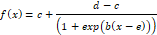
According to Bruce and Versteeg (1992), the logistic model is defined as follows:

Selection Criteria based on Information Measures

In this research, in addition to the widely known criteria to evaluate the goodness of fit of the models, such as the coefficient of determination (R²) and the residual standard error (ERR), there are the information criteria or entropy indices.

Akaike Information Criteria (AIC)

This criterion is detailed in González and Landro (2018), who points out that if the problem consists of selecting the coefficients β that are as close as possible to the vector β* , the distance between the distributions fYβ*  and fYβ  can be characterized by an entropy measure of the form (see Akaike, H. (1978b)):

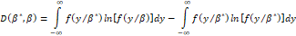
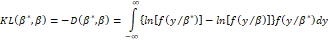
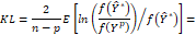
(where the first addend of the second member represents the ability to fit of fYβ  for fYβ*  and the second addend, for a given function fYβ* , is a constant). The minimization of the entropy measure implies the minimization of the information criterion (see Kullback, 1959):

Assuming that β=β*+∆β  (where ∆β=∆β1  ∆β2  …  ∆βk T  is an arbitrary norm vector small), then the criterion KLβ*,β  admits a Taylor series expansion of the form:

If fyβ*  is a regular function, the first term of the second member of this expression vanishes and, consequently, it follows that  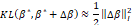(where ∆βI2=∆βTIβ*∆β  , where ⦁I2   is the Euclidean norm and I(⦁) is the information matrix of Fisher). Suppose that β is included in an s-dimensional space Θs1,2,…,k-1 , while the vector of the true values of the coefficients, β* , is included in a k-dimensional space ( k > s). Denoting by βs*   the projection of β*  onΘs  in the sense of the Euclidean norm; it is shown that 2KLβ*,βs≈βs*-β*I2+βs-βs*I2  (where βs∈Θs  and it is verified that βs≈βs* ).

Replacing βs  by the vector of random variables βs  formed by the restricted maximum-likelihood estimators of β*  in Θs  and, taking into account that, for values of n that are sufficiently large, , it is verified that 2EKLβ*,βs≈βs*-β*I2+sn 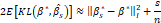. This expression constitutes a measure of the deviations of βs  to the vector β*  and allows us to conclude that the expected value of this deviation includes a component that represents the error related to the selection of a coefficient space approximated by βs*   and another which represents the error due to the estimation of the vector of the coefficients. Akaike showed that, under certain conditions of regularity, the likelihood ratio is:

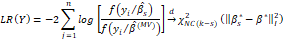
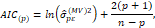
And therefore, that  is an unbiased estimator of the measure EKLβ*-βs . The Akaike information criterion (AIC) consists of minimizing the logarithm of the likelihood function -2LnY,βs+2s   s=1,2…,k-1  in which the first term represents the measure of the error due to the lack of capacity to adapt to the approximation and the second term defines the penalty factor. Under the assumption of normality of the assumed true model, its density function assumes the form:

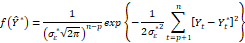
and the likelihood function of the candidate model Ytp  will be of the form. Therefore, the Kullback-Leibler distance will assume the form:

1-…-∅pYt-p2.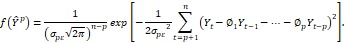

Hence, the Kullback-Leibler distance will assume the form:

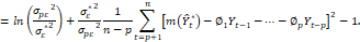
Thus, substituting in this expression the coefficients ∅j , σε*2  ^ 2 and σpε2   by their maximum-likelihood estimators, we obtain:

From this definition the following selection criteria results:

which allows obtaining an asymptotically efficient estimator .

Bootstrapping Estimation

In addition to the maximum likelihood estimators of the parameters of the nonlinear models considered in this investigation, the estimation was performed using the Bootstrap method proposed by Efron (1979), which is one of the simplest methods used to obtain an estimator of a parameter β=β(P)  where P is the postulated statistical model. Alonso (2001) presents the Bootstrap method in a general situation:

Let be Z = (Z1, Z2, ..., Zn)  a data set generated by the statistical model P, and let be T(Z) the statistic whose distribution L(T ; P) we wish to estimate. The Bootstrap method proposes as an estimator of L(T ; P) the distribution L*(T*; n Pˆ ) of the statistic T* =T (Z*), where Z* is a data set generated by the estimated model Pn . Note that if Pn=P , then the distributions L(T; P) and L*(T*; Pn)  coincide. Then if we have a good estimator of P, it is logical to suppose that L*(T*; Pn)  it will approach L(T ; P).

The models described above, their estimators (EMV & Bootstrap), and the model selection criteria (AIC & ERR) were determined in the R environment, using the “drc” package and the “boot” package (R Core Team 2020). For details see Appendixes 1 and 2.

Results

Table 1 shows the results of the evaluation of entropy in three non-linear models (exponential, logistic & Gompertz) adjusted to data from confirmed cases of contagion by COVID-19 in Peru in the period March 6 - April 15, 2020, and related statistics. There it is observed that, for each of the models considered, the entropy index (AIC) and the residual standard error (ERR) increase as the sample size increases (days considered in the study). In the same way, the variances σβi2  of the maximum likelihood estimators (EMV) of the peak of the curve (c in the case of the exponential model and d in the Gompertz & logistic models) increase when n grows, which results in unstable estimators, even when the data shows a good fit, especially in the case of the logistic model (see Figure 1). On the other hand, Figure 2 shows a comparison of the estimates by maximum likelihood and Bootstrap of the peak of confirmed cases of contagion by COVID-19. There it is observed that the Bootstrap estimators show a better performance than the EMV, as well as a considerable increase in their value on day 35. However, for values ​​of n ≤ 10 the EMV show a better performance than the Bootstrap estimators.

Discussion

About the results of the entropy measurement of the models, Cuestas, (2013) points out that entropy is related to the information generation rate, hence the increase in the AIC and EER values ​​associated with the three models as n grows, it may be related to the rate of generation of official information expressed in the differential of the number of rapid and molecular tests applied. Regarding the Bootstrap estimators, Quintana (2003) points out that the error of the Bootstrap approximation to the distribution of the pivotal Tn  is of order n-1  in probability, so the Bootstrap can not only allow approximating the probabilistic distribution statistics of interest when obtaining it is complex, but also allows to improve the normal approximation of the classical estimators, among them the EMV. In this sense, this may explain the performance of the Bootstrap estimators against the EMV when n grows, and in turn, the behavior of the EMV against the Bootstrap estimators when n ≤ 10.

Table 1. Evaluation of the Entropy of Non-linear Models Adjusted to the Data of Confirmed Cases of Contagion by COVID-19 in Peru between March 6 - April 15, 2020.

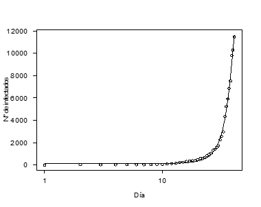
Figure 1. Adjusted Logistic Model on the Data from Confirmed Cases of COVID-19 Infection in Peru (March 6- April 15, 2020).

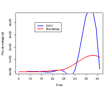
Figure 2. Maximum Likelihood Estimate vs. Bootstrap of the Peak of Contagion (d) using a Logistic Model on Data from Confirmed Cases of Contagion by COVID-19 in Peru (March 6-April 15, 2020).

References

Akaike H (1978b) On the likelihood of a time series model. The Statistician. 27: 237-242.
Alonso A (2001) Bootstrap confidence intervals for indicators in regression. Marrow, 10 (1), 11-20.
Alzahrani, M. I., Alzahrani, M. I., Alsolami, E. A., Al Sulami, A. H., Abdulrahman, A., Alhejaili, M. A. A.
Bruce RD, & Versteeg DJ (1992) A statistical procedure for modeling continuous toxicity data. Environ. Toxicol. Chem, 11(1), 1485–1494.
Cuesta E. (2013). Predictability of the spatial and temporal spread of the AH1N1 influenza epidemic in Argentina. Available at: http://lildbi.fcm.unc.edu.ar/lildbi/tesis/cuestas_eduardo_jose.pdf
Efron B. (1979). Bootstrap methods: Another look at the jackknife. Annals of Statistic. 7(1): 1- 26.
González C. (2016). Statistical significance and p-values. Cuban Journal of Hygiene and Epidemiology, 54(3), 60-62.
González M, & Landro A. (2018). Information criteria and stochastic complexity. Journal of Research in Financial Models, 7(1), 21-40.
Kullback S. (1959). Information theory and statistics. New York: Wiley.
Lu H, Stratton CW, & Tang Y. (2020) Outbreak of pneumonia of unknown etiology in Wuhan China: the mystery and the miracle. J. Med. Virol, 92(4), 401-402.
National Institute of Health [Internet]. Lima: INS; 2020 [cited 2020 Apr 9]. Available at: https://web.ins.gob.pe/
Organization for Economic Cooperation and Development (2006) Current approaches in the statistical analysis of ecotoxicity data: A guidance to application – annexes. Paris: p. 80.
Quintana M. (2003) Bootstrap estimation with sequential data. [Doctoral Thesis]. Spain: Department of Mathematics, University of Las Palmas de Gran Canaria; 2003.Available at: https://accedacris.ulpgc.es/bitstream/10553/19572/4/0287981_00000_0000.pdf
R Core Team (2020) R Development Core Team. R: A language and environment for statistical computing. Disponible en: http://www.r-project.org, http://www.bioassay.dk
Seber GA, & Wild CJ. (1989) Nonlinear Regression, New York: Wiley & Sons.
Sundus, A., Ismail, N. E., & Gnanasan, S. (2018). Exploration of healthcare practitioner’s perception regarding pharmacist’s role in cancer palliative care, Malaysia. Pharmacophore, 9(4), 1-7.
World Health Organization (2019) Technical Focus: Early Clinical and Epidemiological Investigations on COVID-19 for a Public Health Response; 2019. [Internet] [cited 2020 Apr 9]; Available at: https://www.who.int/emergencies/diseases/novel‐coronavirus‐2019/technical‐guidance/early‐investigations.
World Health Organization, WHO Director-General’s Remarks at the Media Briefing on 2019-nCoV. 2020.[Internet]. [citado 08 de abril de 2020]; Disponible en: https://www.who.int/dg/speeches/ detail/who-director-general-s-remarks-at-the-media-briefing-on-2019-ncov-on-11- february-2020.